Machine Learning Part 6
As I have mentioned several times, there is a problem with the training algorithm where I have been processing each digit one by one. Instead, I should have been leveraging matrix math and processing batches of images in a single operation. It’s now time to tackle this problem. But first some bike shedding / procrastination. I gave NetworkConfig a work over.
Layers
The way layers are defined in the network configuration has up to now been a bit meh. There has been a list of “layers” which is a count of the neurons in each layer and a separate list of activation functions.
pub struct NetworkConfig {
    /// Sizes of each layer in the network, including input and output layers.
    /// For example, `[784, 128, 10]` represents a network with:
    /// - 784 input neurons
    /// - 128 hidden neurons
    /// - 10 output neurons
    pub layers: Vec<usize>,

    /// Activation types for each layer transition.
    /// The length should be one less than the number of layers.
    /// Each activation function is applied to the output of its corresponding layer.
    pub activations: Vec<ActivationType>,
    ...
These have been combined. There is now a Layer struct that has the neuron count (called nodes for some reason ) and the activation function (ActivationType) for a layer.
pub struct Layer {
    /// The number of nodes (neurons) in this layer.
    pub nodes: usize,
    /// The activation function applied to the output of this layer.
    /// If `None`, no activation function is applied (e.g., for the output layer).
    pub activation: Option<ActivationType>,
}
activation is an Option because the last layer, the output, doesn’t have an activation function. I also added impl fmt::Display for Layer so they are printed nicely. See the stats output later in this post. NetworkConfig now has a list of Layers
pub struct NetworkConfig {
    /// A collection of [`Layer`]s in the network, including input and output layers.
    /// For example,
    /// vec![Layer { nodes: 784, activation: Some(ActivationType::Sigmoid) },
    ///      Layer { nodes: 128, activation: Some(ActivationType::Sigmoid) },
    ///      Layer { nodes: 10, activation: None }]
    /// represents a network with:
    /// - 784 input neurons (e.g., 28x28 pixels) with sigmoid activation
    /// - 128 hidden neurons with sigmoid activation
    /// - 10 output neurons with no activation
    pub layers: Vec<Layer>,
    ...
The network configuration JSON file now looks like this
{
  "layers": [
    { "nodes": 784, "activation": "Sigmoid" },
    { "nodes": 128, "activation": "Softmax" },
    { "nodes": 10 }
  ],
  "learning_rate": 0.01,
  "epochs": 30,
  "batch_size": 32
}
This was a partial refactor. Network still has the original seperate lists. NetworkConfig has two functions that Network uses to get the layer info. I’ll add Layer to Network at a later time.
Newtypes
I have created newtypes for the configuration parameters. Newtypes look like this.
pub struct Momentum(f64);
We wrap the bare type, the f64, in a tuple struct. Then we can either create a constructor and a value accessor or we implement Try/From which is a bit like a type cast.
impl TryFrom<f64> for Momentum {
    type Error = &'static str;

    fn try_from(value: f64) -> Result<Self, Self::Error> {
        if (0.0..1.0).contains(&value) {
            Ok(Self(value))
        } else {
            Err("Momentum must be between 0.0 and 1.0")
        }
    }
}

impl From<Momentum> for f64 {
    fn from(momentum: Momentum) -> Self {
        momentum.0
    }
}
We define functions that convert from one type to the other and we use TryFrom because it could fail. We can also add methods to our type just like any otherstruct. This trait is for the multiplication operator (*). This is how you define an operator in Rust. Always strike me as a bit weird.
impl Mul<Momentum> for f64 {
    type Output = f64;

    fn mul(self, momentum: Momentum) -> Self::Output {
        self * momentum.0
    }
}
And you use these new types like this
let momentum: Momentum = Momentum::try_from(0.5).unwrap()

let my_float: f64 = f64::from(momentum);
This does a few things
- Makes sure you don’t create an invalid value. Momentums should be between 0.0 and 1.0. The code will fail if the value is outside this range.
- Makes sure the value you pass into a function is actually the momentum value and not some other
f64value. Rust doesn’t have named arguments so you could easily pass in your arguments out of order. - Makes sure your type only has the methods that make sense.
This might seem like it’s expensive converting between these types all the time, but (I’m pretty sure) the compiler removes all this. The new types are there to ensure I don’t mess up and the compiler, once it’s confirmed I haven’t, will strip all these type conversions from the executable.
This is the secondary benefit of this whole process. I’m getting a deeper understanding of Rust and it might be edging out Ruby as my favourite programming language.
Big Matrices
On to the big problem; processing the images in bulk.
Almost all of the code so far has been dealing with single column matrices (vectors?). The MNIST code generates a big list of 784x1 matrices and those get passed around and, as already discussed, eventually processed individually. What I really want are matrices of 784x(a large number) that get passed into the feed forward and back propagation functions and use ndarray to operate on multidimensional matrices. Mathematically there’s (almost) no difference between multiplying 1 or 1000 column matrices.
It took quite a bit of heading scratching but in the end it was a fairly simple change. It only really impacted the process_batch function. Rather than iterating over the list of matrices like this
    fn process_batch(&mut self, batch_inputs: &[&Matrix], batch_targets: &[&Matrix]) -> (f64, usize, Vec<Matrix>) {
        let mut accumulated_gradients = Vec::new();
        let mut batch_error = 0.0;
        let mut batch_correct = 0;

        // Process each sample in the batch
        for (input, target) in batch_inputs.iter().zip(batch_targets.iter()) { // <--- BAD!
            let outputs = self.feed_forward((*input).clone());
I concatenated the functions inputs into two big matrices and got rid of the inner loop.
    fn process_batch(&mut self, batch_inputs: Vec<&Matrix>, batch_targets: Vec<&Matrix>) -> (f64, usize) {
        // Combine batch inputs and targets into single matrices
        let input_matrix = Matrix::concatenate(&batch_inputs, Axis(1));
        let target_matrix = Matrix::concatenate(&batch_targets, Axis(1));

        // Feed forward entire batch at once
        let outputs = self.feed_forward_batch(input_matrix);
Then we pass these multi-column matrices through the functions that already took a single column matrix. For example feed_forward takes a Matrix as a parameter. Before the matrix was a single column, now it’s a 784xbatch_size matrix. I didn’t need to change this code at all.
fn feed_forward(&mut self, inputs: Matrix) -> Matrix {
Eventually they get to ndarray which figures out how to deal with multi-column matrices. I said in Part 3 that I expected this to improve the performance. I was not wrong.
Creating network...
Network Configuration:
  Layer 0: { nodes: 784, activation: Some(Sigmoid) }
  Layer 1: { nodes: 128, activation: Some(Softmax) }
  Layer 2: { nodes: 10, activation: None }
  Learning Rate: 0.0100
  Momentum:      0.5000
  Epochs:        30
  Batch Size:    32
Training network...
  [00:01:01] [################################################################################] 30/30 epochs | Accuracy: Final accuracy: 100.00%
Training completed in 61.222866792s
Total training time: 1m 1s (61.22s)


Confusion Matrix:
      Predicted →
Actual     0    1    2    3    4    5    6    7    8    9
  ↓   +--------------------------------------------------
  0   |  972    0    2    1    0    0    2    1    1    1
  1   |    0 1125    2    2    0    1    3    1    1    0
  2   |    4    0 1008    7    3    0    0    5    5    0
  3   |    0    0    2  996    0    2    0    4    2    4
  4   |    2    1    0    0  961    1    5    0    2   10
  5   |    3    0    0    7    0  874    2    0    4    2
  6   |    3    2    0    1    3    5  941    1    2    0
  7   |    2    3    6    4    0    0    0 1007    0    6
  8   |    3    1    2    3    2    5    1    3  952    2
  9   |    2    2    0    4    9    1    0    4    3  984

Per-digit Metrics:
Digit  | Accuracy | Precision | Recall  | F1 Score
-------|----------|-----------|---------|----------
   0   |  99.2%   |   98.1%   |  99.2%  |   98.6%
   1   |  99.1%   |   99.2%   |  99.1%  |   99.2%
   2   |  97.7%   |   98.6%   |  97.7%  |   98.1%
   3   |  98.6%   |   97.2%   |  98.6%  |   97.9%
   4   |  97.9%   |   98.3%   |  97.9%  |   98.1%
   5   |  98.0%   |   98.3%   |  98.0%  |   98.1%
   6   |  98.2%   |   98.6%   |  98.2%  |   98.4%
   7   |  98.0%   |   98.1%   |  98.0%  |   98.1%
   8   |  97.7%   |   97.9%   |  97.7%  |   97.8%
   9   |  97.5%   |   97.5%   |  97.5%  |   97.5%

Overall Accuracy: 98.20%
Processing time is now down to one minute! And after hanging around 97% for this entire series the test set is consistently at 98% accuracy.
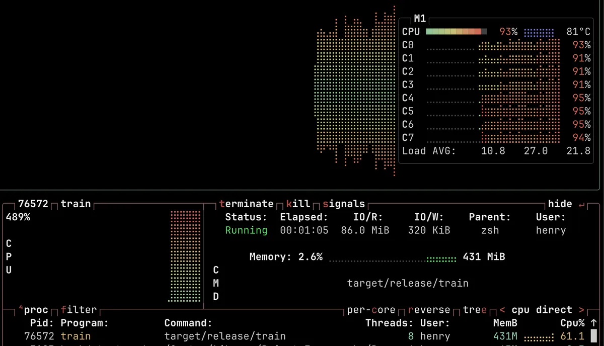
I said in Part 4 that I saw no evidence of multi treading. Well these changes have changed that too. Training is getting more than 400% CPU utilisation now. So those big matrices are being spread across the CPU cores which is nice to see. I can also hear it too which is a bit disconcerting. There’s a definite electrical hum from my iMac when I run the training.
This is very satisfying for a couple of reasons. When I started this series the code took 20 minutes to produce the output shown on the first post. And now the code is looking much nicer.